6. Functions and their properties; Trigonometric functions $\sin(\theta)$ and $\cos(\theta)$ PDF
Functions
Functions
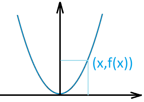
Functions. A function \(f:X \to Y\) is a relation from \(X\) to \(Y\) with the property that for every \(x \in X\) there is a unique element \(y \in Y\) such that \(xRy\) in which case we write \[y=f(x).\]
Example 1. \(X=\mathbb{R}\), \(f(x)=x^2\).
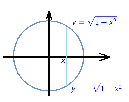
A relation which is not a function
Example 2. \[D=\{(x,y) \in \mathbb{R}^2\;:\;x^2+y^2=1\}.\] This is not a function!
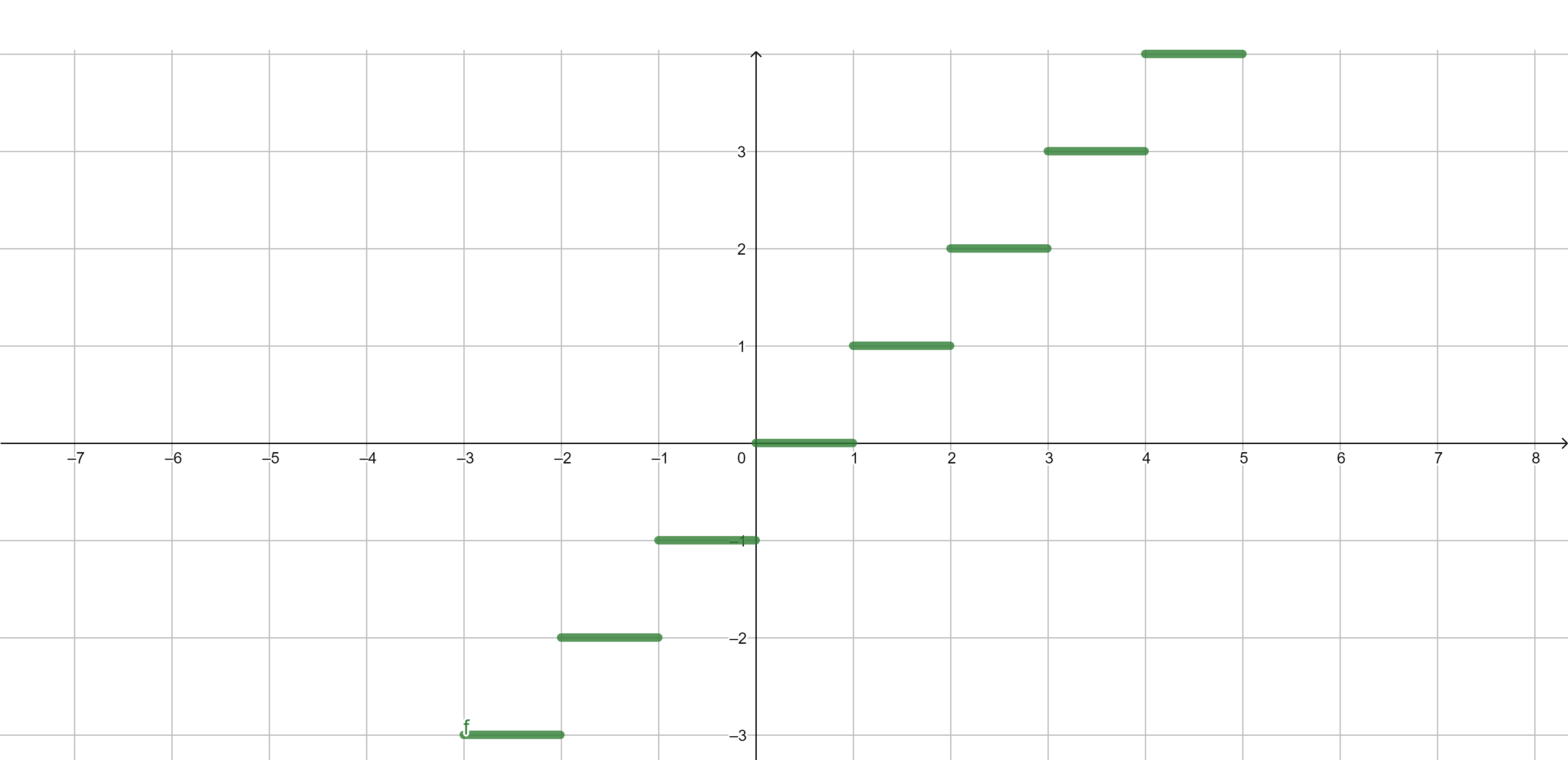
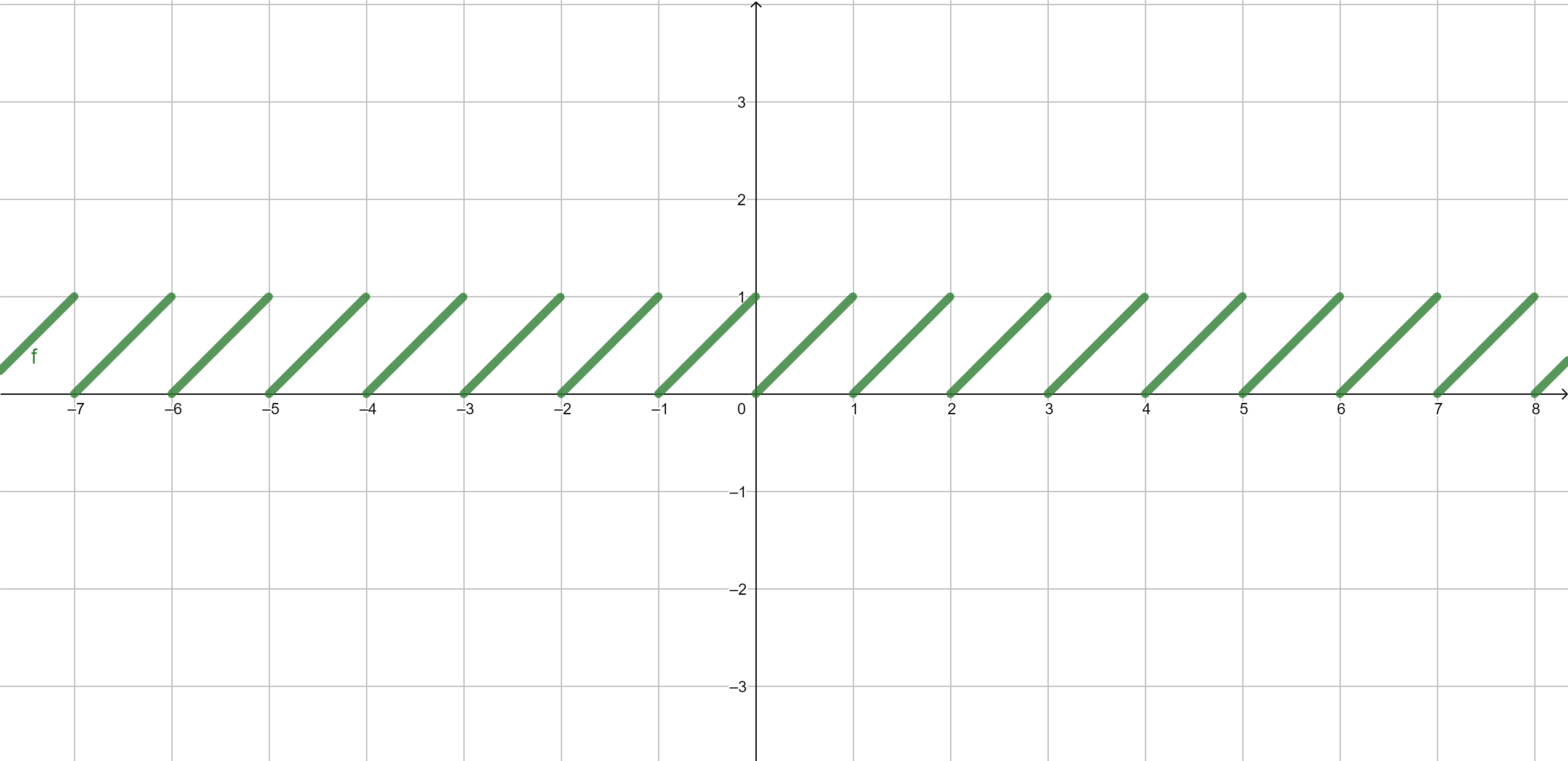
Examples of functions - integer part
Integer part \[\lfloor x\rfloor=\max\{n \in \mathbb{Z}:n \leq x\}.\]
Examples of functions - fractional part
Fractional part \[\{x\}=x-\lfloor x\rfloor.\]
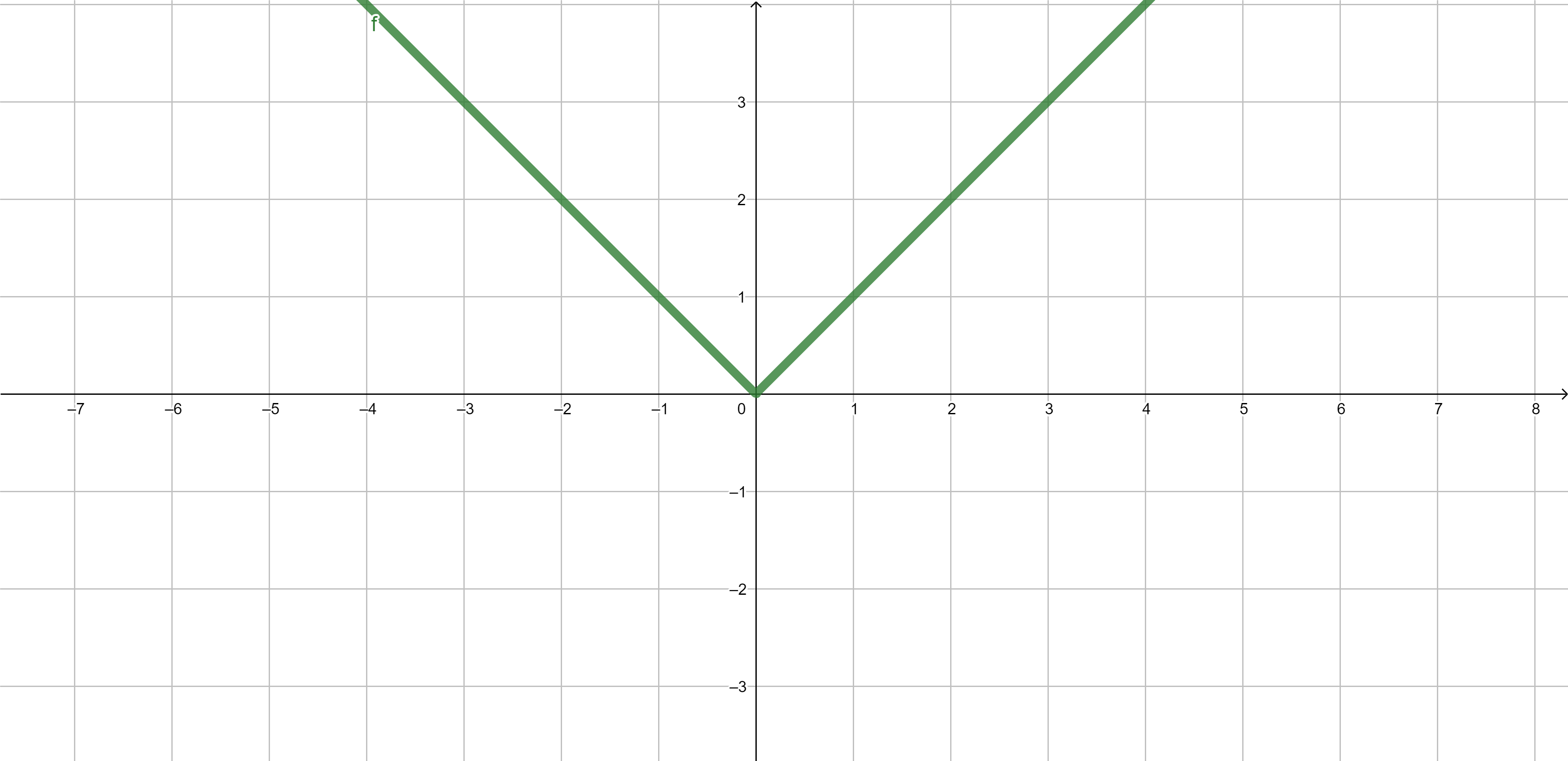
Examples of functions - absolute value
Absolute value \[|x|=\begin{cases} x & \text{ if }x\geq 0,\\ -x & \text{ if }x<0. \end{cases}.\]
Properties of functions
Composition of functions
Composition of functions. If \(f:X \to Y\) and \(g:Y \to Z\) are functions we define their composition \(g \circ f:X \to Z\) by setting \[g \circ f(x)=g(f(x)) \quad \text{ for } \quad x\in X.\]
Example. If \(f(x)=x^2-2\) and \(g(x)=|x|\), then \(g \circ f(x)=|x^2-2|\).
Composition of the functions - example
\[{\color{olive}f(x)=x^2-2}, \qquad {\color{red}g(x)=|x|,}\] \[{\color{blue}g \circ f(x)=|x^2-2|}\]
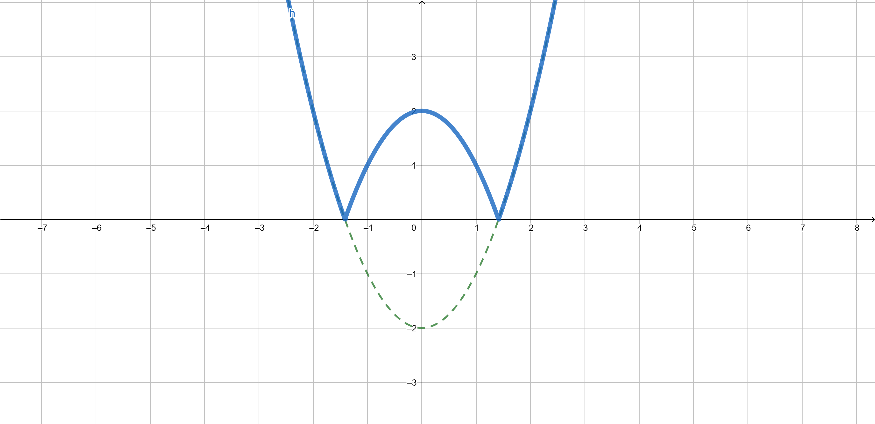
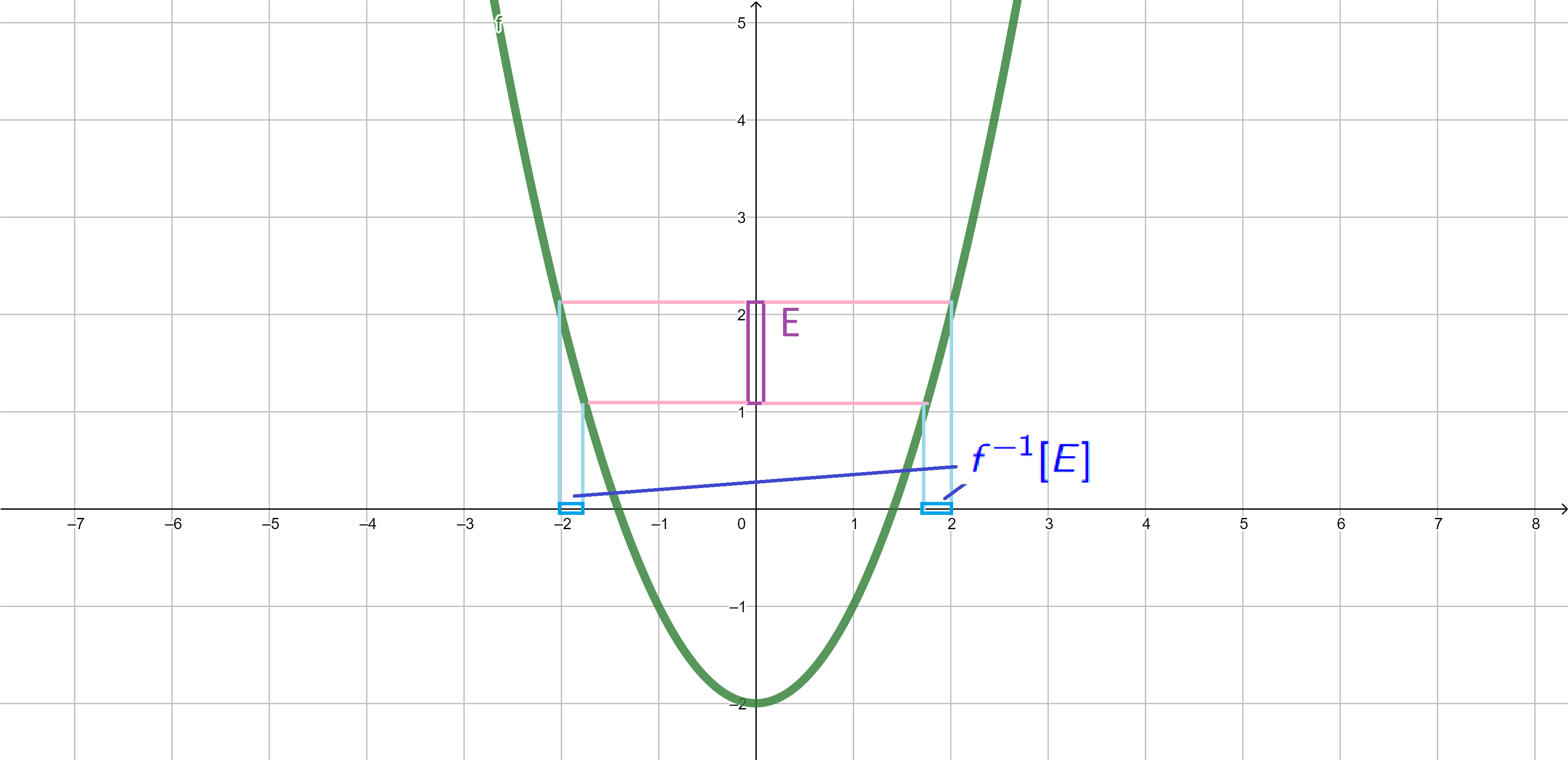
Image and inverse image
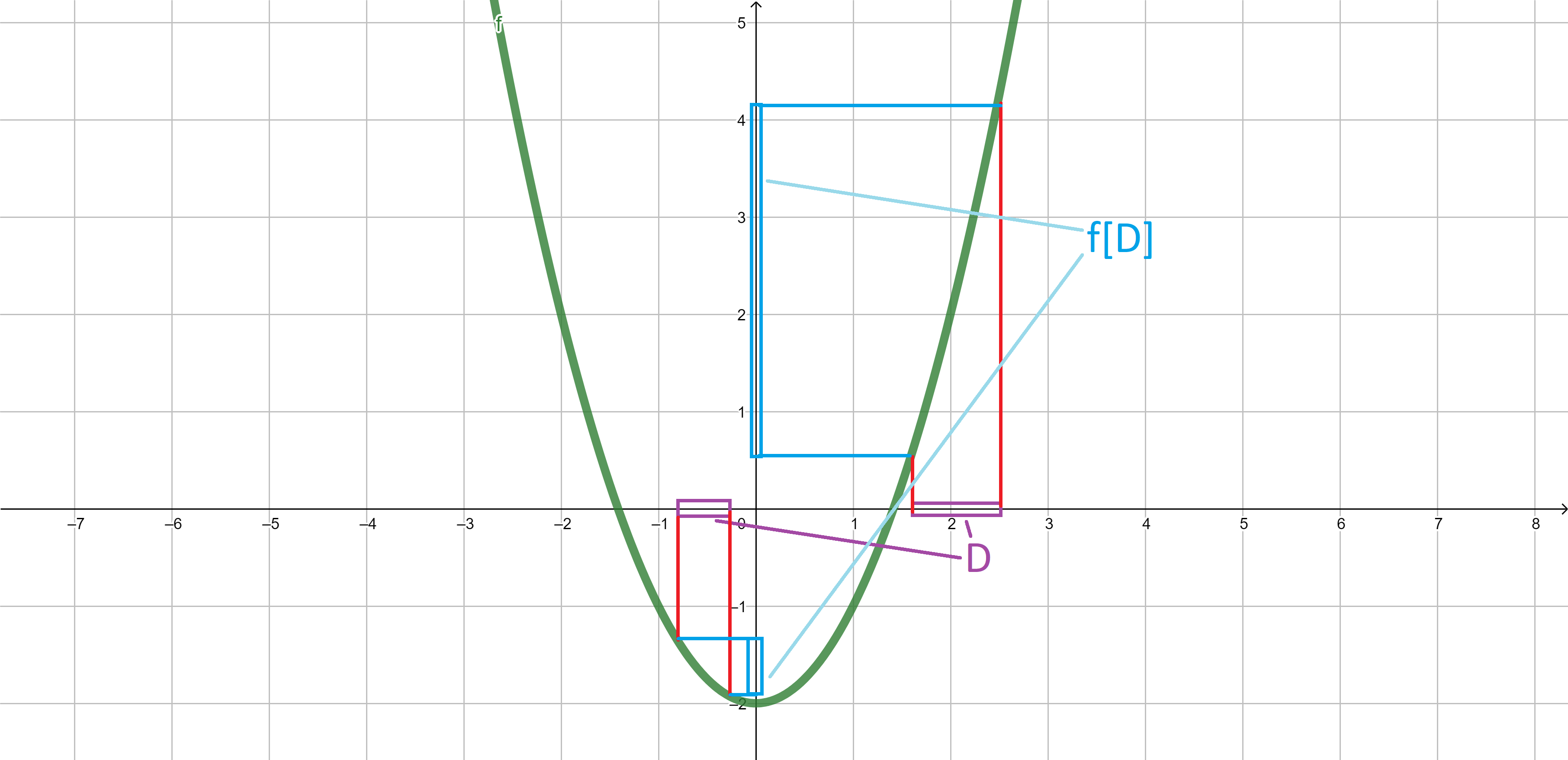
Image. If \(D \subseteq X\), we define the image of \(D\) under the function \(f:X \to Y\) by \[f[D]=\{f(x)\;:\;x \in D\}.\]
Inverse image. If \(E \subseteq Y\), we define the inverse image of \(E\) under the function \(f:X \to Y\) by \[f^{-1}[E]=\{x \in X\;:\;f(x) \in E\}.\]
Image - example
\[{\color{blue}f[D]}=\{f(x)\;:\;x \in {\color{purple}D}\}.\]
Inverse image - example
\[{\color{blue}f^{-1}[E]}=\{x \in X\;:\;f(x) \in {\color{purple}E}\}.\]
Inverse image - properties
For every function \(f:X\to Y\) one has
\[f^{-1}\left[\bigcup_{\alpha \in A}E_{\alpha}\right]=\bigcup_{\alpha \in A}f^{-1}[E_{\alpha}],\]
\[f^{-1}\left[\bigcap_{\alpha \in A}E_{\alpha}\right]=\bigcap_{\alpha \in A}f^{-1}[E_{\alpha}],\]
\[f^{-1}[E^{c}]=(f^{-1}[E])^{c}.\]
Image - properties
For every function \(f:X\to Y\) one has
\[f\left[\bigcup_{\alpha \in A}E_{\alpha}\right]=\bigcup_{\alpha \in A}f[E_{\alpha}].\]
Exercise. Corresponding formulas for intersection and complements may not be true.
Domain and range
Domain. If \(f: X \to Y\) is a function, \(X\) is called the domain of \(f\) and denoted by \[{\rm dom}(f)=X.\]
Range. If \(f: X \to Y\) is a function, \(f[X]\) is called the range of \(f\) denoted by \[{\rm rgn}(f)=f[X].\]
Example. If \(f:\mathbb{R} \to \mathbb{R}\) and \(f(x)=x^2\), then \[{\rm dom}(f)=\mathbb{R} \qquad \text{ and } \qquad {\rm rgn}(f)=[0,\infty).\]
Injective functions, 1/2
Injective functions. The function \(f\) is said to be injective if \(f(x_1)=f(x_2)\) implies \(x_1=x_2\).
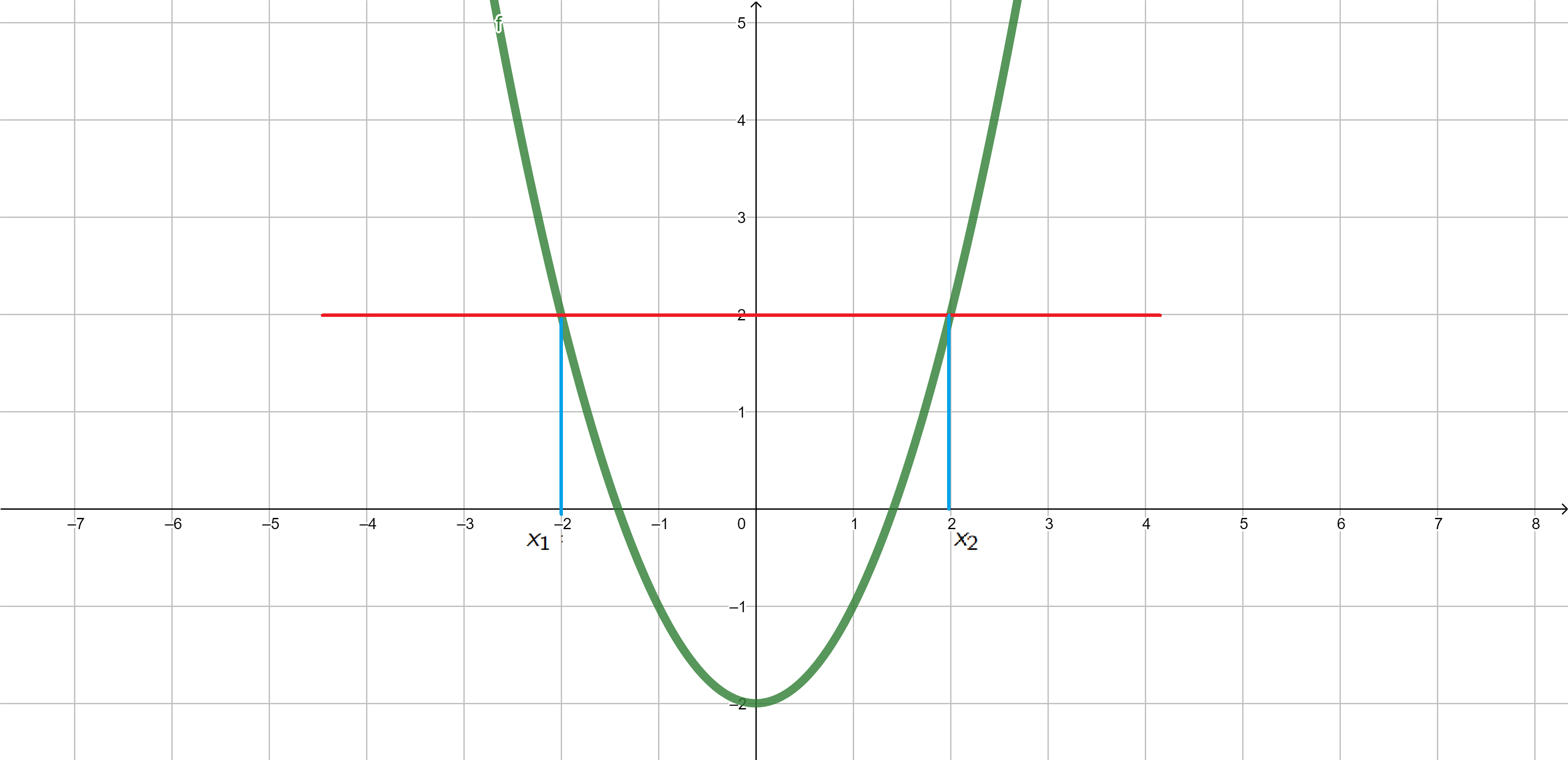
Example 1. \(f(x)=x^2-2\) is not injective since for \(x_1=-2\) and \(x_2=2\) we have \[f(x_1)=f(-2)=(-2)^2-2=2,\]
\[f(x_2)=f(2)=2^2-2=2.\]
Injective functions - example 1/2
\(f(x)=x^2-2\)
Injective functions, 2/2
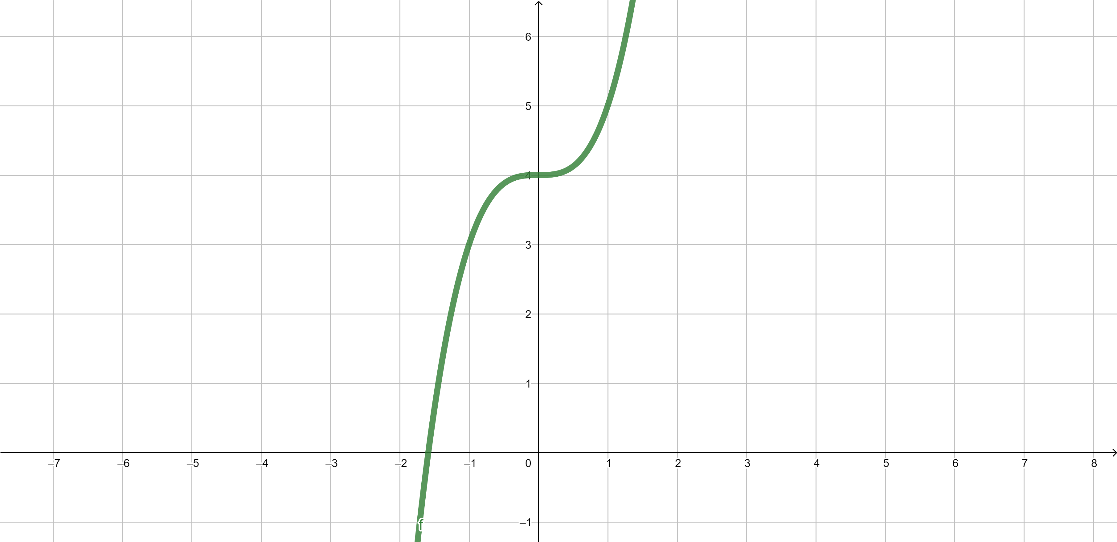
Example 2. \(f(x)=x^3+4\) is injective.
Proof: Indeed, suppose that \(f(x_1)=f(x_2)\), then
\[\begin{aligned} f(x_1)&=f(x_2) \iff\\ x_1^3+4&=x_2^3+4\iff \\ x_1^3&=x_2^3 \iff x_1=x_2. \end{aligned}\]
$$\tag*{$\blacksquare$}$$
Injective functions - example 2/2
\(f(x)=x^3+4\)
Surjective functions
Surjective functions. \(f:X \to Y\) is said to be surjective if \(f[X]=Y\).
Example 1. \(f:\mathbb{R} \to \mathbb{R}\) defined by \(f(x)=x^3-5\) is surjective.
Example 2. \(f:\mathbb{R} \to \mathbb{R}\) defined by \(f(x)=x^2-2\) is not surjective since \[f[\mathbb{R}]=[-2,+\infty) \neq \mathbb{R}.\]
Example 3. Every mapping \(f:X \to Y\) is surjective if \(Y=f[X]\).
Bijective functions
Bijective functions. \(f:X \to Y\) is bijective if it is both injective and surjective.
Example 1. \(f:\mathbb{R} \to \mathbb{R}\) defined by \(f(x)=ax+b\) is bijective is \(a \neq 0\).
Example 2. \(f:\mathbb{R} \to \mathbb{R}\) defined by \(f(x)=x^3+5\) is bijective.
Example 3. \(f:\mathbb{R} \to \mathbb{R}\) defined by \(f(x)=x^2+1\) is not bijective since it is not injective.
Inverse functions
Inverse functions. If \(f:X \to Y\) is bijective it has an inverse \(f^{-1}:Y \to X\) such that \[f^{-1} \circ f \quad \text{ and }\quad f \circ f^{-1}\] are both identity functions, i.e. \[f^{-1} \circ f(x)=x\quad \text{ and }\quad f \circ f^{-1}(y)=y\quad \text{ for all } \quad x \in X, y \in Y.\]
Example 1. If \(a \neq 0\), then \(f(x)=ax+b\) has an inverse given by \[f^{-1}(x)=\frac{x-b}{a}.\]
Restriction of the function
Restriction. If \(A \subseteq X\) we denote \(f_{|A}\) the restriction of \(f:X \to Y\) to \(A\): \[f_{|A}:A \to Y, \qquad f_{|A}(x)=f(x)\qquad \text{ for all } \qquad x \in A.\]
Example 1. Let \(f:\mathbb{R} \to \mathbb{R}\) be defined by \(f(x)=x^2\). Let \(A=[0,+\infty)\) and let \(g(x)=f_{|A}\). Then \(f\) is not injective, but \(g\) is injective.
Trigonometric functions
Angle
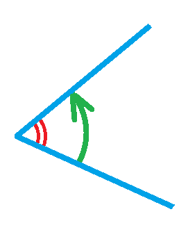
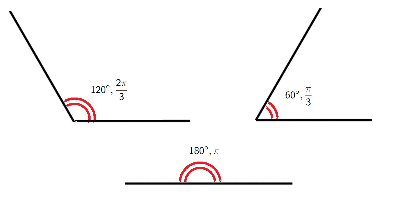
An angle can be thought of as the amount of rotation required to take one straight line to another line with a common endpoint. Angles can be measured in degrees or in radians (abbreviated as rad). The angle given by a complete revolution contains \(360^{\circ}\) and
\[{\color{blue}2\pi {\rm \; rad}=360^{\circ}}\].
Examples
Angle in standard position. An angle is in standard position if its vertex (the endpoint of two rays) is located at the origin and one ray is on the positive \(x\)-axis. The ray on the \(x\)-axis is called the initial side and the other ray is called the terminal side.
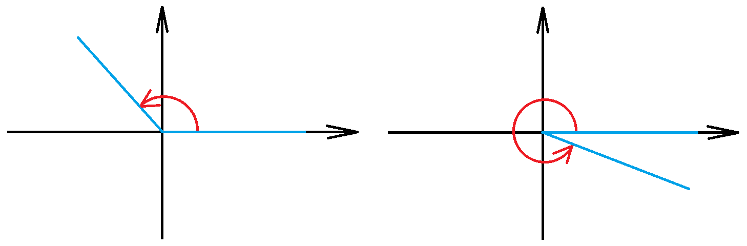
Using this terminology the angle is measured by the amount of rotation from the initial side to the terminal side. If measured in a counterclockwise direction the measurement is positive. If measured in a clockwise direction the measurement is negative.
Example 1
Example 2
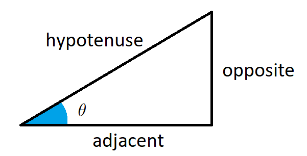
\(\sin(\theta)\) and \(\cos(\theta)\) for acute angle
\(\sin(\theta)\) and \(\cos(\theta)\) for acute angle. For an acute angle \(\theta\) the quantities \({\color{red}\sin(\theta)}\) and \({\color{blue}\cos(\theta)}\) are defined as ratios of lengths of sides of a right triangle as follows \[{\color{red}\sin(\theta)=\frac{\text{opposite}{}}{\text{hypotenuse}}}, \qquad {\color{blue}\cos(\theta)=\frac{\text{adjacent}{}}{\text{hypotenuse}}}.\]
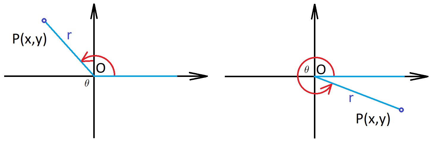
\(\sin(\theta)\) and \(\cos(\theta)\) for any angle
\(\sin(\theta)\) and \(\cos(\theta)\) for any angle. The previous definition does not apply to angles which are not acute, so for a general angle in standard position we let \(P(x,y)\) be any point on the terminal side and we let \(r\) be the distance \(|OP|\) (\(O\) is the origin). Then we define \[{\color{red}\sin(\theta)=\frac{y}{r}}, \qquad {\color{blue}\cos(\theta)=\frac{x}{r}}.\]
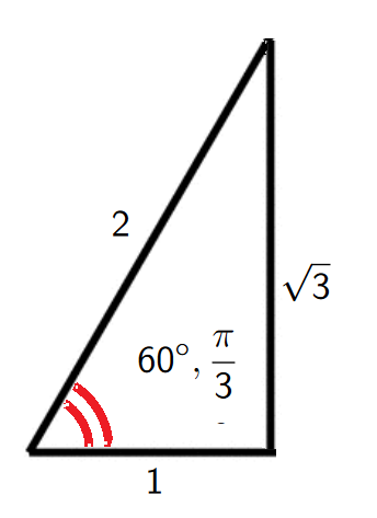
Examples 1
Example 1/4. For an acute angle \(\theta=\frac{\pi}{3}\) we have \[{\color{red}\sin(\theta)=\frac{\sqrt{3}}{2}}, \qquad {\color{blue}\cos(\theta)=\frac{1}{2}}.\]
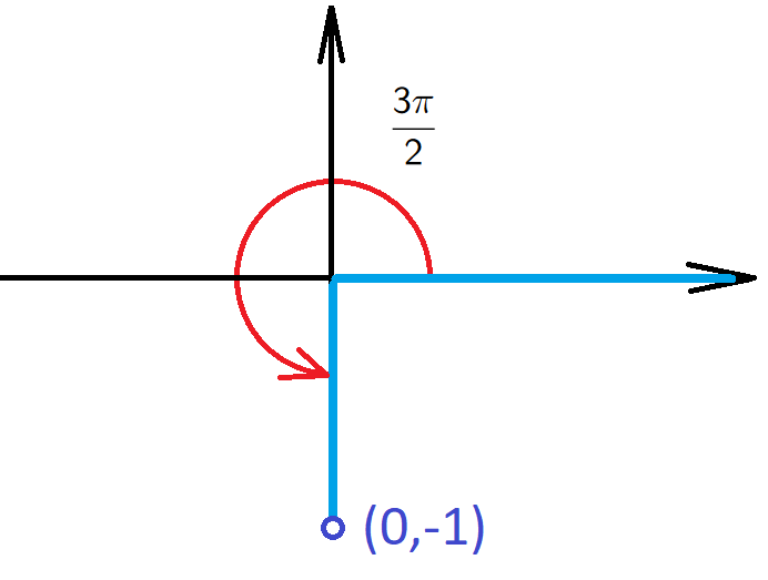
Examples 2/4
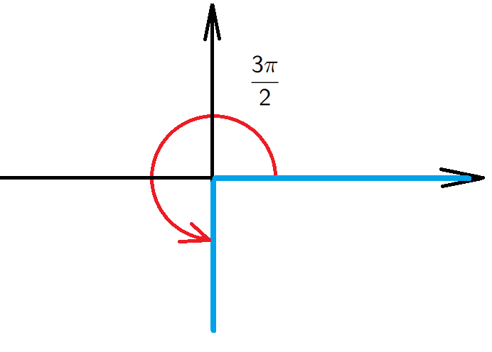
Example 2. For an angle \(\theta=\frac{3\pi}{2}\) we have a point \((0,-1)\) on the terminal side, so \[{\color{red}\sin(\theta)=\frac{-1}{1}=-1}, \qquad {\color{blue}\cos(\theta)=\frac{0}{1}=0}.\]
Examples 3/4
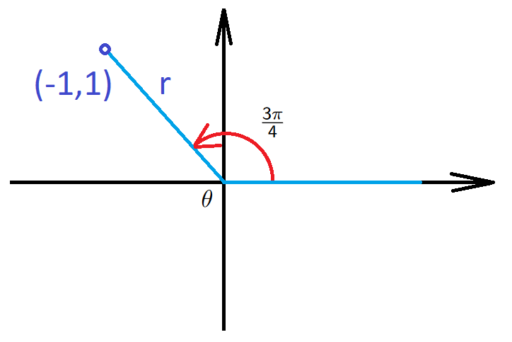
Example 3. For an angle \(\theta=\frac{3\pi}{4}\) we have a point \((-1,1)\) on the terminal side, so \[{\color{red}\sin(\theta)=\frac{1}{\sqrt{2}}=\frac{\sqrt{2}}{2}}, \qquad {\color{blue}\cos(\theta)=\frac{-1}{\sqrt{2}}=-\frac{\sqrt{2}}{2}}.\]
Examples 4/4
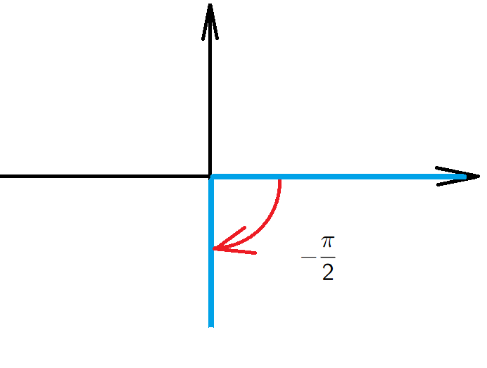
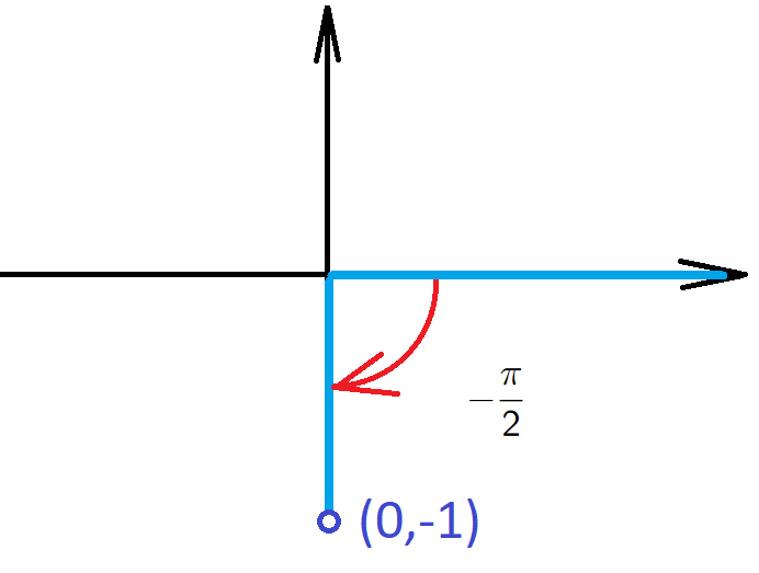
Example 4. For an angle \(\theta=-\frac{\pi}{2}\) we have a point \((0,-1)\) on the terminal side, so \[{\color{red}\sin(\theta)=\frac{-1}{1}=-1}, \qquad {\color{blue}\cos(\theta)=\frac{0}{1}=0}.\]
Values of trigonometric functions
Trigonometric identities
Pythagorean identity. For any angle \(\theta\) we have \[{\color{purple}\sin^2(\theta)+\cos^2(\theta)=1}.\]
Proof. Let \(P(x,y)\) be any point on the terminal side. By the definition of \(\sin(\theta)\) and \(\cos(\theta)\) we have \[\sin^2(\theta)+\cos^2(\theta)=\frac{y^2}{|OP|^2}+\frac{x^2}{|OP|^2}.\] But by the Pythagorean theorem \[|OP|^2=x^2+y^2,\] hence \[\hspace{3cm}\sin^2(\theta)+\cos^2(\theta)=\frac{|OP|^2}{|OP|^2}=1. \hspace{3cm}\tag*{$\blacksquare$}\]
Trigonometric identities. We have the following identities, which can be observed geometrically:
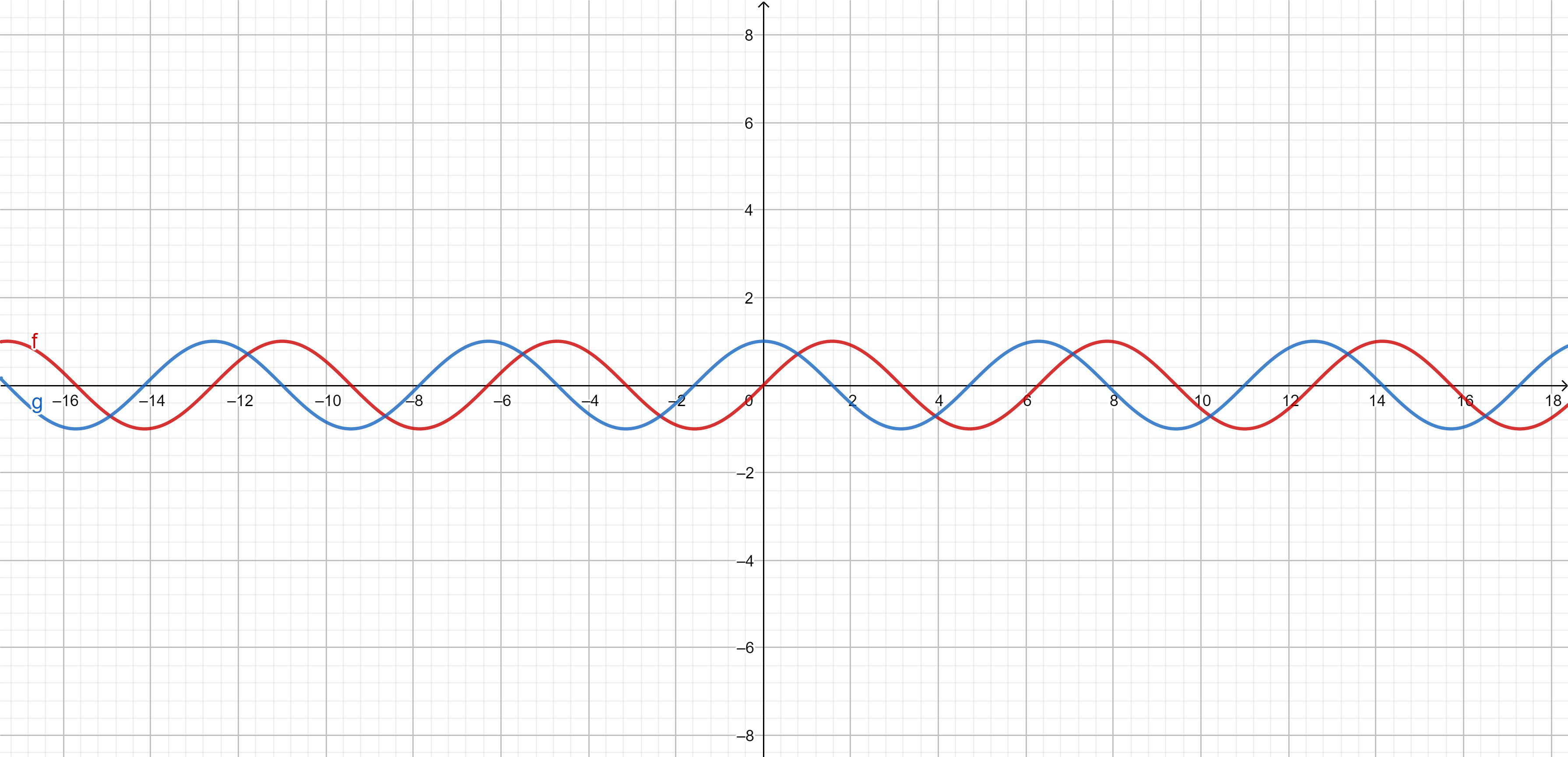
\(\sin(x+\frac{\pi}{2})=\cos(x)\),
\(\cos(x+\frac{\pi}{2})=-\sin(x)\),
\(\sin(x+\pi)=-\sin(x)\),
\(\cos(x+\pi)=-\cos(x)\),
\(\sin(x+2\pi)=\sin(x)\),
\(\cos(x+2\pi)=\cos(x)\).
Graph of \({\color{red}\sin(x)}\) and \({\color{blue}\cos(x)}\)